ANOVA TEST to Determine Statistical Significance

Running ANOVA test to check whether the total value of ATM transactions using debit cards in India is influenced by the month of the year. The data for the analysis has been obtained from the RBI (Reserve Bank of India) database and can be accessed here:

https://www.rbi.org.in/Scripts/ATMView.aspx

In order to make sure the data is in a format fit for analysis, I have reformated the data to look like the following:

http://falcon80.com/Blogs/wp-content/uploads/2016/03/ATMTRANSACTIONS.xlsx

Null Hypothesis: The value of ATM transactions is not influenced by the time of the year.

SAS Code for the ANOVA Test:

/* Generated Code (IMPORT) */
/* Source File: ATMTransactionsIndia.xlsx */
/* Source Path: /home/isabelleraja0 */
/* Code generated on: Sunday, March 13, 2016 2:13:24 AM */

/* Generated Code (IMPORT) */
/* Source File: ATMTRANSVALUE.xlsx */
/* Source Path: /home/isabelleraja0/sasuser.v94 */
/* Code generated on: Sunday, March 13, 2016 10:50:31 PM */

%web_drop_table(WORK.IMPORT);

FILENAME REFFILE “/home/isabelleraja0/sasuser.v94/ATMTRANSACTIONS.xlsx” TERMSTR=CR;

PROC IMPORT DATAFILE=REFFILE
DBMS=XLSX
OUT=WORK.IMPORT;
GETNAMES=YES;
PROC CONTENTS DATA=WORK.IMPORT;

%web_open_table(WORK.IMPORT);
RUN;
LABEL AVERAGE= “Average Value of ATM debit Card Transactions”;

PROC ANOVA; CLASS Month;
MODEL AVERAGE = Month;
MEANS Month;

RUN;

Output:

Dependent Variable: AVERAGE AVERAGE

Source DF Sum of Squares Mean Square F Value Pr > F
Model 11 141511021368 12864638306 0.10 0.9999
Error 44 5.4603717E12 124099357802
Corrected Total 55 5.6018828E12
R-Square Coeff Var Root MSE AVERAGE Mean
0.025261 22.24858 352277.4 1583370
Source DF Anova SS Mean Square F Value Pr > F
Month 11 141511021368 12864638306 0.10 0.9999
Distribution of AVERAGE by Month

The ANOVA Procedure

Distribution of AVERAGE by Month
Level of
Month
N AVERAGE
Mean Std Dev
April 5 1536279.49 375268.096
August 5 1584656.82 379527.519
December 4 1575451.39 284465.328
February 4 1461088.70 203371.834
January 4 1587887.78 307202.647
July 5 1599382.48 379468.261
June 5 1550018.21 354715.995
March 4 1664288.02 290951.425
May 5 1606618.10 391837.800
November 5 1597240.90 366743.451
October 5 1663292.20 388804.856
September 5 1565286.56 381076.242

Inference:

Since the P value =0.99 and is very high, there is not enough evidence to reject the null hypothesis. Since there is not evidence to reject the null hypothesis, there is no need for a post-hoc test.

Posted in Big Data, Data Analysis, Uncategorized | Tagged | Leave a comment

Visualizing Data

Univariate graphs for the 4 variables I have chosen:

Death by Asphyxiation:

Code:

import pandas
import numpy
import math
import matplotlib.pyplot as plt
import seaborn

data = pandas.read_csv(‘data.csv’)

data[‘YISM2534’] = pandas.to_numeric(data[‘YISM2534’])
data[‘YISW2534’] = pandas.to_numeric(data[‘YISW2534’])
data[‘DBA’] = pandas.to_numeric(data[‘DBA’])

data[‘DBACEIL’] = numpy.ceil(data[‘DBAPER1000’])

#data[‘DBACEIL’] = int(data[‘DBAPER1000’])

# Where data is not available, it is coded as 1001.
# We will change the missing data to nan.

data[‘DBACEIL’] = data[‘DBACEIL’].replace(1001,numpy.nan)

DBADescribe = data[‘DBACEIL’].describe()
print(DBADescribe)

#Univariate Graph
seaborn.distplot(data[‘DBACEIL’].dropna(), kde=”false”)
plt.xlabel(‘Death by asphyxiation per 1000’)
plt.title(‘Distribution of death by asphyxiation per 1000’)

Output:
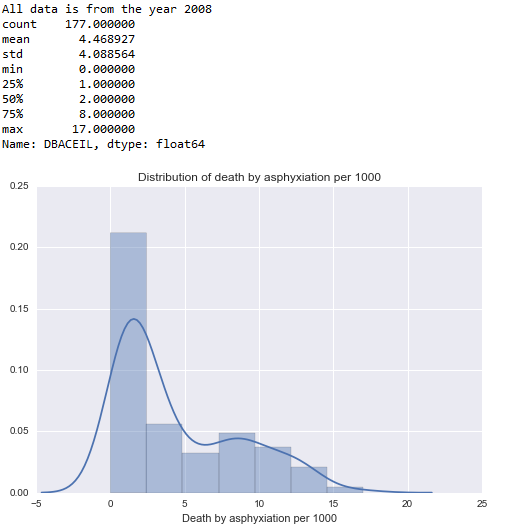
DBA_Univariate

Percentage of births attend by professional staff

Code:

import pandas
import numpy
import math
import matplotlib.pyplot as plt
import seaborn

data = pandas.read_csv(‘data.csv’)

data[‘YISM2534’] = pandas.to_numeric(data[‘YISM2534’])
data[‘YISW2534’] = pandas.to_numeric(data[‘YISW2534’])
data[‘DBA’] = pandas.to_numeric(data[‘DBA’])

print(“Number of rows in the data file” )
print(len(data))
print(“Number of variables”)
print(len(data.columns))

print(“All data is from the year 2008″)

data[‘BIRTHPROSTAFFCEIL’] = numpy.ceil(data[‘BIRTHPROSTAFF’])

# Where data is not available, it is coded as 101.
# We will change the missing data to nan.

data[‘BIRTHPROSTAFFCEIL’] = data[‘BIRTHPROSTAFFCEIL’].replace(101,numpy.nan)

BIRTHPROSTAFFDescribe = data[‘BIRTHPROSTAFFCEIL’].describe();
#print(BIRTHPROSTAFFDescribe)

#Univariate Graph
seaborn.distplot(data[‘BIRTHPROSTAFFCEIL’].dropna(), kde=”false”)
plt.xlabel(‘% of births attended by professional staff’)
plt.title(‘Distribution of % of births attended by professional staff’)

Output:
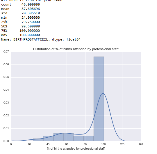
BirthsByProStaff_Univariate

Average Education of Men:

Code:
import pandas
import numpy
import math
import matplotlib.pyplot as plt
import seaborn

data = pandas.read_csv(‘data.csv’)

data[‘YISM2534’] = pandas.to_numeric(data[‘YISM2534’])
data[‘YISW2534’] = pandas.to_numeric(data[‘YISW2534’])
data[‘DBA’] = pandas.to_numeric(data[‘DBA’])

print(“Number of rows in the data file” )
print(len(data))
print(“Number of variables”)
print(len(data.columns))

print(“All data is from the year 2008″)
data[‘YISM2534CEIL’] = numpy.ceil(data[‘YISM2534’])

# Where data is not available, it is coded as 0.
# We will change the missing data to nan.

data[‘YISM2534CEIL’] = data[‘YISM2534CEIL’].replace(0,numpy.nan)

#Univariate Graph
seaborn.distplot(data[‘YISM2534CEIL’].dropna(), kde=”false”)
plt.xlabel(‘Average number of years of education for men between 25 – 34’)
plt.title(‘Distribution of Average number of years of education for men’)

Output:
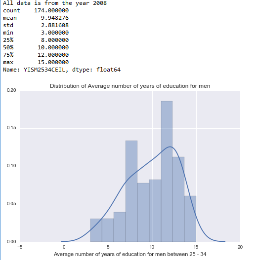
EducationMen_Univariate

Average Education of Women:

Code:

import pandas
import numpy
import math
import matplotlib.pyplot as plt
import seaborn

data = pandas.read_csv(‘data.csv’)

data[‘YISM2534’] = pandas.to_numeric(data[‘YISM2534’])
data[‘YISW2534’] = pandas.to_numeric(data[‘YISW2534’])
data[‘DBA’] = pandas.to_numeric(data[‘DBA’])

print(“Number of rows in the data file” )
print(len(data))
print(“Number of variables”)
print(len(data.columns))

print(“All data is from the year 2008″)

data[‘YISW2534CEIL’] = numpy.ceil(data[‘YISW2534’])
#print(YISM2534FLOOR)

# Where data is not available, it is coded as 0.
# We will change the missing data to nan.

data[‘YISW2534CEIL’] = data[‘YISW2534CEIL’].replace(0,numpy.nan)

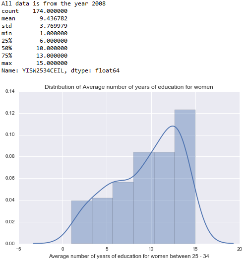
YISW2534Describe = data[‘YISW2534CEIL’].describe();
print(YISW2534Describe)

#Univariate Graph
seaborn.distplot(data[‘YISW2534CEIL’].dropna(), kde=”false”)
plt.xlabel(‘Average number of years of education for women between 25 – 34’)
plt.title(‘Distribution of Average number of years of education for women’)

Output:
YISW2534_univariate

Bivariate Graphs:

Association between death by asphyxiation and % of births attended by professional staff:

Code:
import pandas
import numpy
import math
import matplotlib.pyplot as plt
import seaborn

data = pandas.read_csv(‘data.csv’)

data[‘YISM2534’] = pandas.to_numeric(data[‘YISM2534’])
data[‘YISW2534’] = pandas.to_numeric(data[‘YISW2534’])
data[‘DBA’] = pandas.to_numeric(data[‘DBA’])

print(“Number of rows in the data file” )
print(len(data))
print(“Number of variables”)
print(len(data.columns))

print(“All data is from the year 2008″)

data[‘DBACEIL’] = numpy.ceil(data[‘DBAPER1000’])
data[‘DBACEIL’] = data[‘DBACEIL’].replace(1001,numpy.nan)

data[‘BIRTHPROSTAFFCEIL’] = numpy.ceil(data[‘BIRTHPROSTAFF’])
data[‘BIRTHPROSTAFFCEIL’] = data[‘BIRTHPROSTAFFCEIL’].replace(101,numpy.nan)

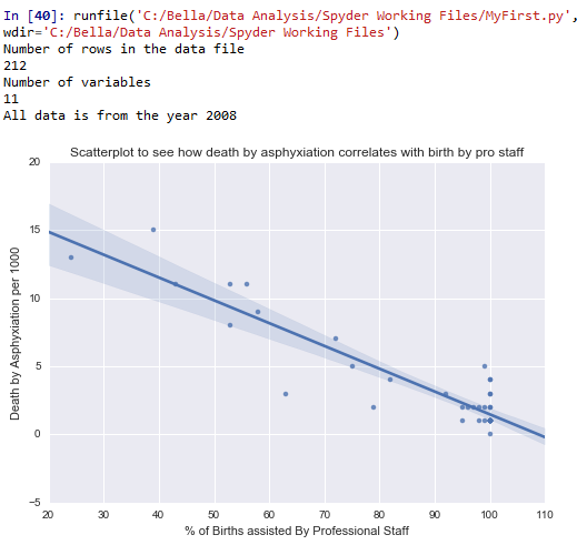
scat1 = seaborn.regplot(x=”BIRTHPROSTAFFCEIL”, y=”DBACEIL”, fit_reg=True, data=data)
plt.xlabel(‘% of Births assisted By Professional Staff’)
plt.ylabel(‘Death by Asphyxiation per 1000’)
plt.title(‘Scatterplot to see how death by asphyxiation correlates with birth by pro staff’)

Output:
1_bivariate

Conclusion: The graph shows a negative correlation between number of deaths by asphyxiation per 1000 and % of births attended by professional staff. This means, the more the births attended by professional staff, the less the number of deaths by asphyxiation. That said, the correlation is not very tight. Part of the problem is also the lack of adequate data for % of births attended by professional staff across countries.

Association between % of births attended by professional staff and average education of men:

Code:
import pandas
import numpy
import math
import matplotlib.pyplot as plt
import seaborn

data = pandas.read_csv(‘data.csv’)

data[‘YISM2534’] = pandas.to_numeric(data[‘YISM2534’])
data[‘YISW2534’] = pandas.to_numeric(data[‘YISW2534’])
data[‘DBA’] = pandas.to_numeric(data[‘DBA’])

print(“Number of rows in the data file” )
print(len(data))
print(“Number of variables”)
print(len(data.columns))

print(“All data is from the year 2008″)

data[‘BIRTHPROSTAFFCEIL’] = numpy.ceil(data[‘BIRTHPROSTAFF’])

# Where data is not available, it is coded as 101.
# We will change the missing data to nan.

data[‘BIRTHPROSTAFFCEIL’] = data[‘BIRTHPROSTAFFCEIL’].replace(101,numpy.nan)

data[‘YISM2534CEIL’] = numpy.ceil(data[‘YISM2534’])

# Where data is not available, it is coded as 0.
# We will change the missing data to nan.

data[‘YISM2534CEIL’] = data[‘YISM2534CEIL’].replace(0,numpy.nan)
# A bivariate graph to check whether death by asphyxiation correlates with birth by pro staff

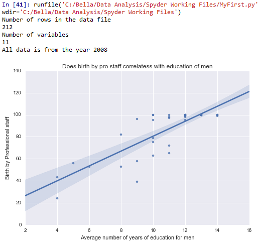
scat2 = seaborn.regplot(x=”YISM2534CEIL”, y=”BIRTHPROSTAFFCEIL”, fit_reg=True, data=data)
plt.xlabel(‘Average number of years of education for men’)
plt.ylabel(‘Birth by Professional staff’)
plt.title(‘Does birth by pro staff correlatess with education of men’)
2_bivariate

Conclusion: When examining whether there is an association between the average education of men between the age group 25 – 34 and whether the women seek professional care during child birth, we see that there is a positive correlation. However, again, this correlation does not seem to be very tight. Nevertheless, the more the men are educated, the more the women in that country tend to seek professional help for child birth.

Association between % of births attended by professional staff and average age of women

Code:

import pandas
import numpy
import math
import matplotlib.pyplot as plt
import seaborn

data = pandas.read_csv(‘data.csv’)

data[‘YISM2534’] = pandas.to_numeric(data[‘YISM2534’])
data[‘YISW2534’] = pandas.to_numeric(data[‘YISW2534’])
data[‘DBA’] = pandas.to_numeric(data[‘DBA’])

print(“Number of rows in the data file” )
print(len(data))
print(“Number of variables”)
print(len(data.columns))

print(“All data is from the year 2008″)

data[‘BIRTHPROSTAFFCEIL’] = numpy.ceil(data[‘BIRTHPROSTAFF’])

# Where data is not available, it is coded as 101.
# We will change the missing data to nan.

data[‘BIRTHPROSTAFFCEIL’] = data[‘BIRTHPROSTAFFCEIL’].replace(101,numpy.nan)

data[‘YISW2534CEIL’] = numpy.ceil(data[‘YISW2534’])
#print(YISM2534FLOOR)

# Where data is not available, it is coded as 0.
# We will change the missing data to nan.

data[‘YISW2534CEIL’] = data[‘YISW2534CEIL’].replace(0,numpy.nan)
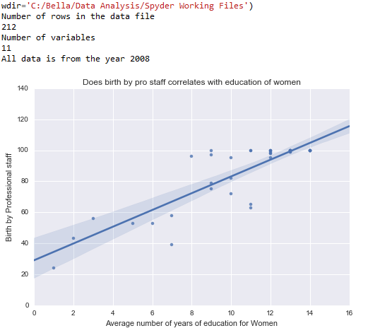
scat3 = seaborn.regplot(x=”YISW2534CEIL”, y=”BIRTHPROSTAFFCEIL”, fit_reg=True, data=data)
plt.xlabel(‘Average number of years of education for Women’)
plt.ylabel(‘Birth by Professional staff’)
plt.title(‘Does birth by pro staff correlates with education of women’)

Output:
3_bivariate

Conclusion: When examining whether there is a relationship between the average number of years of education among women between 25 – 34 and whether they seek professional care during child birth, there seems to be a positive correlation.


Posted in Big Data, Data Analysis | Leave a comment

Data Management

In my previous post, I had performed a frequency analysis on three of the variables from my data set:

YISM2534: Mean years in school (men between 25 and 34 years old)

YISW2534: Mean years in school (women between 25 and 34 years old)

DBA:  Asphyxia deaths in newborn (total deaths)

The analysis was not friendly to interpretation due to the variables taking infinite number of values. Therefore, I have made some changes to the data to make it more interpretable.

  1. First, I have also included a fourth variable for my analysis:  BIRTHPROSTAFF: Total number of births attended by professional staff. I have included BIRTHPROSTAFF as it pertains directly to my primary research question.
  2. Second, I have changed the variable DBA to DBAPer1000 (death by asphyxia per 1000) since this variable accounts for the variations in population size among the different countries whereas DBA does not do so.
  3. Third, I have set aside missing data in each of the variables
    1. YISM2534: Missing data was coded as 0. It has been changed to nan.
    2. YISF2534: Missing data was coded as 0. It has been changed to nan.
    3. DBAPER1000: Missing data was coded as 1001. It has been changed to nan.
    4. BIRTHPROSTAFF: Missing data was coded as 101. It has been changed to nan.
  4. Since each of the variables took infinite number of values (float), frequency analysis did not yield any meaningful data in the earlier run. Therefore, to make the frequency analysis more meaningful, I created secondary variables for each of my chosen variables. The secondary variables are basically the ceiling values of the primary variables. After the conversion, YISM2534 and YISW2534 now take integer values from 1 to 15 without decimals. Similarly, I applied the ceiling function to DBAPER1000 and BIRTHPROSTAFF. This exercise has yielded a more interpretable frequency and percentage analysis for all variables.
  5. I have created a new data frame dataNew using the secondary variables. In my output, I have printed the first 25 rows of this new data frame.
  6. There are no skip patterns in my data set and therefore there is no need to manage skip patterns
  7. All variables take quantitative values and therefore coded logically. Therefore, none of them required recoding.

Code:

# -*- coding: utf-8 -*-
“””
Spyder Editor

This is a temporary script file.
“””
# This is my “Hello World Code”

import pandas
import numpy
import math

data = pandas.read_csv(‘data.csv’)

#data[‘YISM2534’] = data[‘YISM2534’].convert_objects(convert_numeric=True)
#data[‘YISW2534’] = data[‘YISW2534’].convert_objects(convert_numeric=True)
#data[‘DBA’] = data[‘DBA’].convert_objects(convert_numeric=True)

data[‘YISM2534’] = pandas.to_numeric(data[‘YISM2534’])
data[‘YISW2534’] = pandas.to_numeric(data[‘YISW2534’])
data[‘DBA’] = pandas.to_numeric(data[‘DBA’])

print(“Number of rows in the data file” )
print(len(data))
print(“Number of variables”)
print(len(data.columns))

print(“All data is from the year 2008”)

#——————————————————————

data[‘DBACEIL’] = numpy.ceil(data[‘DBAPER1000’])

# Where data is not available, it is coded as 1001.
# We will change the missing data to nan.

data[‘DBACEIL’] = data[‘DBACEIL’].replace(1001,numpy.nan)

print(“Frequency of countries in terms of death by asphyxiation per 1000.”)
DBAFREQ = data[‘DBACEIL’].value_counts(sort=False, dropna=False)
print(DBAFREQ)

print(“Percentage of countries in terms of death by asphyxiation per 1000.”)
DBAPercentage = data[‘DBACEIL’].value_counts(sort=False, dropna=False) * 100 / len (data)
print(DBAPercentage)

#——————————————————————–

data[‘BIRTHPROSTAFFCEIL’] = numpy.ceil(data[‘BIRTHPROSTAFF’])

# Where data is not available, it is coded as 101.
# We will change the missing data to nan.

data[‘BIRTHPROSTAFFCEIL’] = data[‘BIRTHPROSTAFFCEIL’].replace(101,numpy.nan)

print(“Frequency of countries in terms of births attended by professional staff.”)
BIRTHPROSTAFFFREQ = data[‘BIRTHPROSTAFFCEIL’].value_counts(sort=False, dropna=False)
print(BIRTHPROSTAFFFREQ)

print(“Percentage of countries in terms of births attended by professional staff.”)
BIRTHPROSTAFFPercentage = data[‘BIRTHPROSTAFFCEIL’].value_counts(sort=False, dropna=False) * 100 / len (data)
print(BIRTHPROSTAFFPercentage)

#—————————————————————–
data[‘YISM2534CEIL’] = numpy.ceil(data[‘YISM2534’])

# Where data is not available, it is coded as 0.
# We will change the missing data to nan.

data[‘YISM2534CEIL’] = data[‘YISM2534CEIL’].replace(0,numpy.nan)

print(“Frequency of countries in terms of the average number of years of school including primary, secondary and tertiary education attended by all men between 25 and 34 years.”)
YISM2534FREQ = data[‘YISM2534CEIL’].value_counts(sort=False, dropna=False)
print(YISM2534FREQ)

print(“Percentage of countries in terms of the average number of years of school including primary, secondary and tertiary education attended by all men between 25 and 34 years.”)
YISM2534Percentage = data[‘YISM2534CEIL’].value_counts(sort=False, dropna=False) * 100 / len (data)
print(YISM2534Percentage)

#—————————————————————-

data[‘YISW2534CEIL’] = numpy.ceil(data[‘YISW2534’])
#print(YISM2534FLOOR)

# Where data is not available, it is coded as 0.
# We will change the missing data to nan.

data[‘YISW2534CEIL’] = data[‘YISW2534CEIL’].replace(0,numpy.nan)

print(“Frequency of countries in terms of the average number of years of school including primary, secondary and tertiary education attended by all women between 25 and 34 years.”)
YISW2534FREQ = data[‘YISW2534CEIL’].value_counts(sort=False, dropna=False)
print(YISW2534FREQ)

print(“Percentage of countries in terms of the average number of years of school including primary, secondary and tertiary education attended by all women between 25 and 34 years.”)
YISW2534Percentage = data[‘YISW2534CEIL’].value_counts(sort=False, dropna=False) * 100 / len (data)
print(YISW2534Percentage)

#———————————————————————

# Print the new dataframe that contains the ceiling values

dataNew = data[[‘Countries’,’YISM2534CEIL’, ‘YISW2534CEIL’, ‘DBACEIL’, ‘BIRTHPROSTAFFCEIL’ ]]
print(dataNew.head(25))

#———————————————————————-

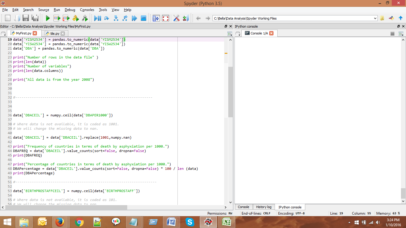
code3

Output:

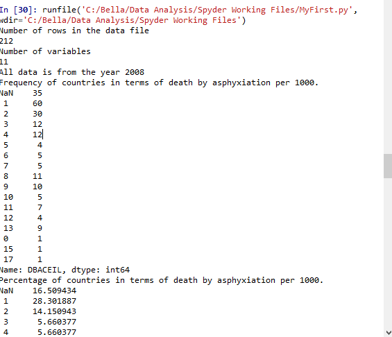
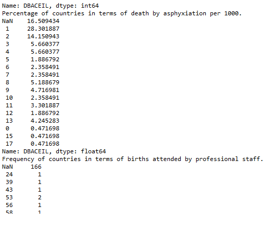
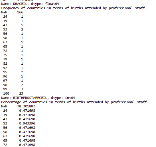
Code3_1 Code3_2 Code3_3 Code3_4 Code3_5 Code3_6 Code3_7 Code3_8

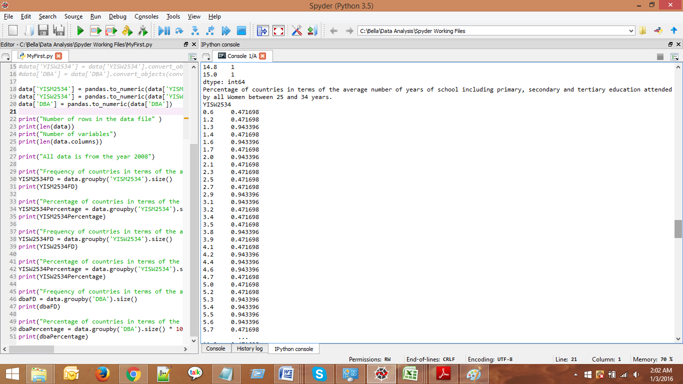
Now that the data has been managed, the frequency analysis on each of the variables is more interpretable. For example, when considering  death by asphyxia per 1000 data, the majority of the countries have a low number –  60 countries have only one recorded death per 1000, 30 countries have only 2 recorded deaths per 1000 and so on. The frequency analysis similarly show meaningful data for the other selected variables.

Output in case the screenshot is not clear:

runfile(‘C:/Bella/Data Analysis/Spyder Working Files/MyFirst.py’, wdir=’C:/Bella/Data Analysis/Spyder Working Files’)
Number of rows in the data file
212
Number of variables
11
All data is from the year 2008
Frequency of countries in terms of death by asphyxiation per 1000.
NaN    35
1     60
2     30
3     12
4     12
5      4
6      5
7      5
8     11
9     10
10     5
11     7
12     4
13     9
0      1
15     1
17     1
Name: DBACEIL, dtype: int64
Percentage of countries in terms of death by asphyxiation per 1000.
NaN    16.509434
1     28.301887
2     14.150943
3      5.660377
4      5.660377
5      1.886792
6      2.358491
7      2.358491
8      5.188679
9      4.716981
10     2.358491
11     3.301887
12     1.886792
13     4.245283
0      0.471698
15     0.471698
17     0.471698
Name: DBACEIL, dtype: float64
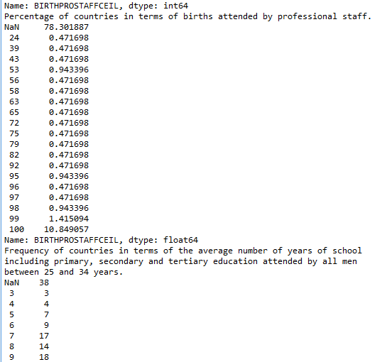
Frequency of countries in terms of births attended by professional staff.
NaN     166
24       1
39       1
43       1
53       2
56       1
58       1
63       1
65       1
72       1
75       1
79       1
82       1
92       1
95       2
96       1
97       1
98       2
99       3
100     23
Name: BIRTHPROSTAFFCEIL, dtype: int64
Percentage of countries in terms of births attended by professional staff.
NaN     78.301887
24      0.471698
39      0.471698
43      0.471698
53      0.943396
56      0.471698
58      0.471698
63      0.471698
65      0.471698
72      0.471698
75      0.471698
79      0.471698
82      0.471698
92      0.471698
95      0.943396
96      0.471698
97      0.471698
98      0.943396
99      1.415094
100    10.849057
Name: BIRTHPROSTAFFCEIL, dtype: float64
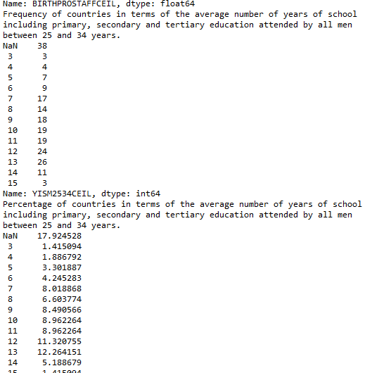
Frequency of countries in terms of the average number of years of school including primary, secondary and tertiary education attended by all men between 25 and 34 years.
NaN    38
3      3
4      4
5      7
6      9
7     17
8     14
9     18
10    19
11    19
12    24
13    26
14    11
15     3
Name: YISM2534CEIL, dtype: int64
Percentage of countries in terms of the average number of years of school including primary, secondary and tertiary education attended by all men between 25 and 34 years.
NaN    17.924528
3      1.415094
4      1.886792
5      3.301887
6      4.245283
7      8.018868
8      6.603774
9      8.490566
10     8.962264
11     8.962264
12    11.320755
13    12.264151
14     5.188679
15     1.415094
Name: YISM2534CEIL, dtype: float64
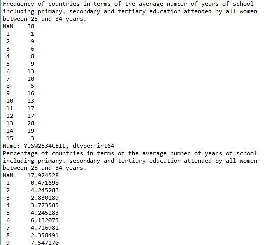
Frequency of countries in terms of the average number of years of school including primary, secondary and tertiary education attended by all women between 25 and 34 years.
NaN    38
1      1
2      9
3      6
4      8
5      9
6     13
7     10
8      5
9     16
10    13
11    17
12    17
13    28
14    19
15     3
Name: YISW2534CEIL, dtype: int64
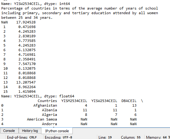
Percentage of countries in terms of the average number of years of school including primary, secondary and tertiary education attended by all women between 25 and 34 years.
NaN    17.924528
1      0.471698
2      4.245283
3      2.830189
4      3.773585
5      4.245283
6      6.132075
7      4.716981
8      2.358491
9      7.547170
10     6.132075
11     8.018868
12     8.018868
13    13.207547
14     8.962264
15     1.415094
Name: YISW2534CEIL, dtype: float64
Countries  YISM2534CEIL  YISW2534CEIL  DBACEIL  \
0              Afghanistan             4             1       13
1                  Albania            11            11        1
2                  Algeria             8             7        6
3           American Samoa           NaN           NaN      NaN
4                  Andorra           NaN           NaN      NaN
5                   Angola             7             5       13
6      Antigua and Barbuda            14            14      NaN
7                Argentina            12            12        1
8                  Armenia            12            12        3
9                    Aruba           NaN           NaN      NaN
10               Australia            13            13        1
11                 Austria            13            12        1
12              Azerbaijan            13            13        4
13                 Bahamas            12            13        2
14                 Bahrain            11            12        1
15              Bangladesh             6             5       10
16                Barbados           NaN           NaN        2
17                 Belarus            13            13        1
18                 Belgium            13            14        1
19                  Belize            10            10        2
20                   Benin             5             3        8
21                 Bermuda           NaN           NaN      NaN
22                  Bhutan           NaN           NaN        9
23                 Bolivia            11            10        7
24  Bosnia and Herzegovina            11            10        2

BIRTHPROSTAFFCEIL
0                  24
1                 NaN
2                 NaN
3                 NaN
4                 NaN
5                 NaN
6                 100
7                  95
8                 100
9                 NaN
10                NaN
11                NaN
12                NaN
13                NaN
14                 98
15                NaN
16                NaN
17                100
18                NaN
19                 95
20                NaN
21                NaN
22                NaN
23                 72
24                NaN

Posted in Uncategorized | Leave a comment

Getting started with Python!

So this week, I wrote my first program in Python for analyzing frequency distribution of data. Unfortunately, the data I had selected did not lend well to frequency distribution. The main reason for this was that none of the variables in the data set was categorical. Therefore the results are not very meaningful at this point. Nevertheless, my first program did run without any errors and displayed the intended results.

My program:

# -*- coding: utf-8 -*-
“””
Spyder Editor

This is a temporary script file.
“””
# This is my “Hello World Code”

import pandas
import numpy

data = pandas.read_csv(‘data.csv’)

#data[‘YISM2534’] = data[‘YISM2534’].convert_objects(convert_numeric=True)
#data[‘YISW2534’] = data[‘YISW2534’].convert_objects(convert_numeric=True)
#data[‘DBA’] = data[‘DBA’].convert_objects(convert_numeric=True)

data[‘YISM2534’] = pandas.to_numeric(data[‘YISM2534’])
data[‘YISW2534’] = pandas.to_numeric(data[‘YISW2534’])
data[‘DBA’] = pandas.to_numeric(data[‘DBA’])

print(“Number of rows in the data file” )
print(len(data))
print(“Number of variables”)
print(len(data.columns))

print(“All data is from the year 2008”)

print(“Frequency of countries in terms of the average number of years of school including primary, secondary and tertiary education attended by all men between 25 and 34 years.”)
YISM2534FD = data.groupby(‘YISM2534’).size()
print(YISM2534FD)

print(“Percentage of countries in terms of the average number of years of school including primary, secondary and tertiary education attended by all men between 25 and 34 years.”)
YISM2534Percentage = data.groupby(‘YISM2534’).size() * 100 / len(data)
print(YISM2534Percentage)

print(“Frequency of countries in terms of the average number of years of school including primary, secondary and tertiary education attended by all Women between 25 and 34 years.”)
YISW2534FD = data.groupby(‘YISW2534’).size()
print(YISW2534FD)

print(“Percentage of countries in terms of the average number of years of school including primary, secondary and tertiary education attended by all Women between 25 and 34 years.”)
YISW2534Percentage = data.groupby(‘YISW2534’).size() * 100 / len(data)
print(YISW2534Percentage)

print(“Frequency of countries in terms of the average number of deaths in new born due to asphyxia.”)
dbaFD = data.groupby(‘DBA’).size()
print(dbaFD)

print(“Percentage of countries in terms of the average number of deaths in new born due to asphyxia.”)
dbaPercentage = data.groupby(‘DBA’).size() * 100 / len(data)
print(dbaPercentage)

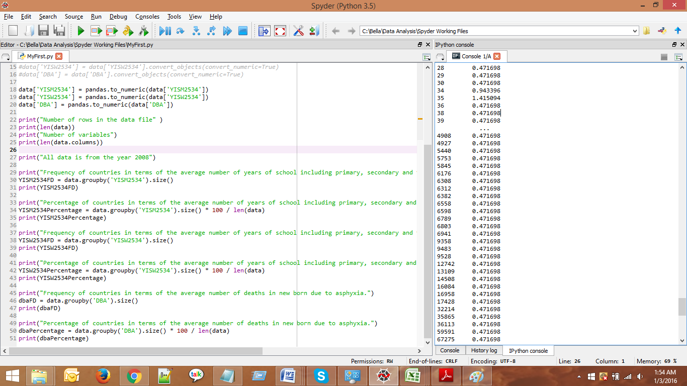
Screen shot of the program

Screenshot1

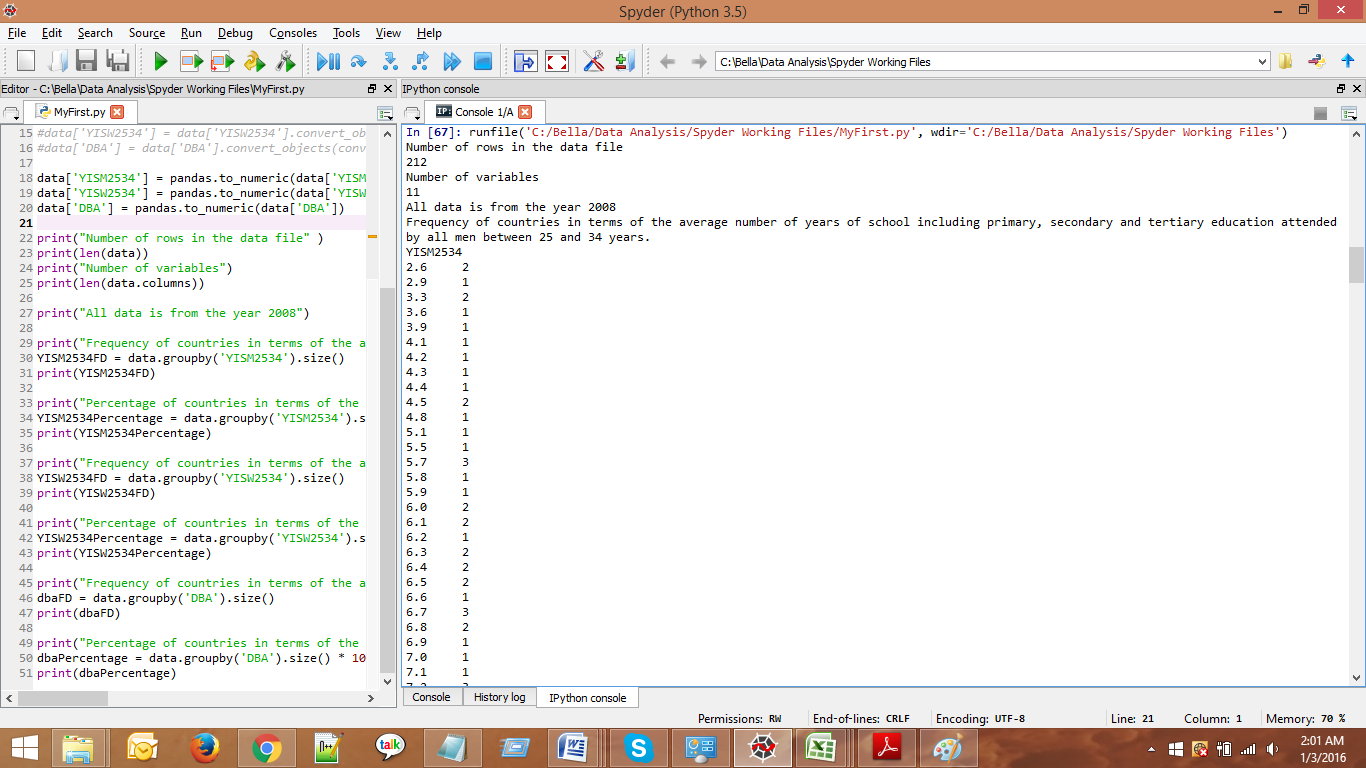
Results

runfile(‘C:/Bella/Data Analysis/Spyder Working Files/MyFirst.py’, wdir=’C:/Bella/Data Analysis/Spyder Working Files’)

Number of rows in the data file

212

Number of variables

11

All data is from the year 2008

Frequency of countries in terms of the average number of years of school including primary, secondary and tertiary education attended by all men between 25 and 34 years.

YISM2534

2.6     2

2.9     1

3.3     2

3.6     1

3.9     1

4.1     1

4.2     1

4.3     1

4.4     1

4.5     2

4.8     1

5.1     1

5.5     1

5.7     3

5.8     1

5.9     1

6.0     2

6.1     2

6.2     1

6.3     2

6.4     2

6.5     2

6.6     1

6.7     3

6.8     2

6.9     1

7.0     1

7.1     1

7.2     3

7.3     3

..

10.7    4

10.9    2

11.0    2

11.1    1

11.2    5

11.3    4

11.4    1

11.5    3

11.7    2

11.9    3

12.0    5

12.1    3

12.2    3

12.3    2

12.4    5

12.5    3

12.6    3

12.8    1

12.9    3

13.0    3

13.1    2

13.2    1

13.3    1

13.4    3

13.5    1

13.6    2

13.7    1

14.3    1

14.7    1

14.8    1

dtype: int64

Percentage of countries in terms of the average number of years of school including primary, secondary and tertiary education attended by all men between 25 and 34 years.

YISM2534

2.6     0.943396

2.9     0.471698

3.3     0.943396

3.6     0.471698

3.9     0.471698

4.1     0.471698

4.2     0.471698

4.3     0.471698

4.4     0.471698

4.5     0.943396

4.8     0.471698

5.1     0.471698

5.5     0.471698

5.7     1.415094

5.8     0.471698

5.9     0.471698

6.0     0.943396

6.1     0.943396

6.2     0.471698

6.3     0.943396

6.4     0.943396

6.5     0.943396

6.6     0.471698

6.7     1.415094

6.8     0.943396

6.9     0.471698

7.0     0.471698

7.1     0.471698

7.2     1.415094

7.3     1.415094


10.7    1.886792

10.9    0.943396

11.0    0.943396

11.1    0.471698

11.2    2.358491

11.3    1.886792

11.4    0.471698

11.5    1.415094

11.7    0.943396

11.9    1.415094

12.0    2.358491

12.1    1.415094

12.2    1.415094

12.3    0.943396

12.4    2.358491

12.5    1.415094

12.6    1.415094

12.8    0.471698

12.9    1.415094

13.0    1.415094

13.1    0.943396

13.2    0.471698

13.3    0.471698

13.4    1.415094

13.5    0.471698

13.6    0.943396

13.7    0.471698

14.3    0.471698

14.7    0.471698

14.8    0.471698

dtype: float64

Frequency of countries in terms of the average number of years of school including primary, secondary and tertiary education attended by all Women between 25 and 34 years.

YISW2534

0.6     1

1.2     1

1.3     2

1.4     1

1.6     2

1.7     1

2.0     2

2.1     1

2.3     1

2.5     1

2.7     1

2.9     2

3.1     2

3.2     1

3.4     1

3.5     1

3.8     2

3.9     1

4.1     1

4.2     2

4.4     2

4.6     2

4.7     1

5.0     1

5.2     1

5.3     2

5.4     2

5.5     2

5.6     2

5.7     1

..

11.3    1

11.4    2

11.5    3

11.6    3

11.7    1

11.8    3

11.9    1

12.0    2

12.1    4

12.2    3

12.3    3

12.4    4

12.5    3

12.6    3

12.7    1

12.8    2

12.9    2

13.0    3

13.1    3

13.2    2

13.3    3

13.4    1

13.5    2

13.6    1

13.7    3

13.8    3

13.9    1

14.5    1

14.8    1

15.0    1

dtype: int64

Percentage of countries in terms of the average number of years of school including primary, secondary and tertiary education attended by all Women between 25 and 34 years.

YISW2534

0.6     0.471698

1.2     0.471698

1.3     0.943396

1.4     0.471698

1.6     0.943396

1.7     0.471698

2.0     0.943396

2.1     0.471698

2.3     0.471698

2.5     0.471698

2.7     0.471698

2.9     0.943396

3.1     0.943396

3.2     0.471698

3.4     0.471698

3.5     0.471698

3.8     0.943396

3.9     0.471698

4.1     0.471698

4.2     0.943396

4.4     0.943396

4.6     0.943396

4.7     0.471698

5.0     0.471698

5.2     0.471698

5.3     0.943396

5.4     0.943396

5.5     0.943396

5.6     0.943396

5.7     0.471698


11.3    0.471698

11.4    0.943396

11.5    1.415094

11.6    1.415094

11.7    0.471698

11.8    1.415094

11.9    0.471698

12.0    0.943396

12.1    1.886792

12.2    1.415094

12.3    1.415094

12.4    1.886792

12.5    1.415094

12.6    1.415094

12.7    0.471698

12.8    0.943396

12.9    0.943396

13.0    1.415094

13.1    1.415094

13.2    0.943396

13.3    1.415094

13.4    0.471698

13.5    0.943396

13.6    0.471698

13.7    1.415094

13.8    1.415094

13.9    0.471698

14.5    0.471698

14.8    0.471698

15.0    0.471698

dtype: float64

Frequency of countries in terms of the average number of deaths in new born due to asphyxia.

DBA

0         1

1         4

2         2

3         1

4         5

6         1

7         2

8         3

9         1

11        1

12        2

13        1

14        2

15        1

16        2

17        1

20        1

21        2

22        1

23        2

24        1

26        3

28        1

29        1

30        1

34        2

35        3

36        1

38        1

39        1

..

4908      1

4927      1

5440      1

5753      1

5845      1

6176      1

6308      1

6312      1

6382      1

6558      1

6598      1

6789      1

6803      1

6941      1

9358      1

9483      1

9528      1

12742     1

13109     1

14508     1

16084     1

16958     1

17428     1

32214     1

35865     1

36113     1

59591     1

67275     1

84990     1

189447    1

dtype: int64

Percentage of countries in terms of the average number of deaths in new born due to asphyxia.

DBA

0         0.471698

1         1.886792

2         0.943396

3         0.471698

4         2.358491

6         0.471698

7         0.943396

8         1.415094

9         0.471698

11        0.471698

12        0.943396

13        0.471698

14        0.943396

15        0.471698

16        0.943396

17        0.471698

20        0.471698

21        0.943396

22        0.471698

23        0.943396

24        0.471698

26        1.415094

28        0.471698

29        0.471698

30        0.471698

34        0.943396

35        1.415094

36        0.471698

38        0.471698

39        0.471698


4908      0.471698

4927      0.471698

5440      0.471698

5753      0.471698

5845      0.471698

6176      0.471698

6308      0.471698

6312      0.471698

6382      0.471698

6558      0.471698

6598      0.471698

6789      0.471698

6803      0.471698

6941      0.471698

9358      0.471698

9483      0.471698

9528      0.471698

12742     0.471698

13109     0.471698

14508     0.471698

16084     0.471698

16958     0.471698

17428     0.471698

32214     0.471698

35865     0.471698

36113     0.471698

59591     0.471698

67275     0.471698

84990     0.471698

189447    0.471698

dtype: float64

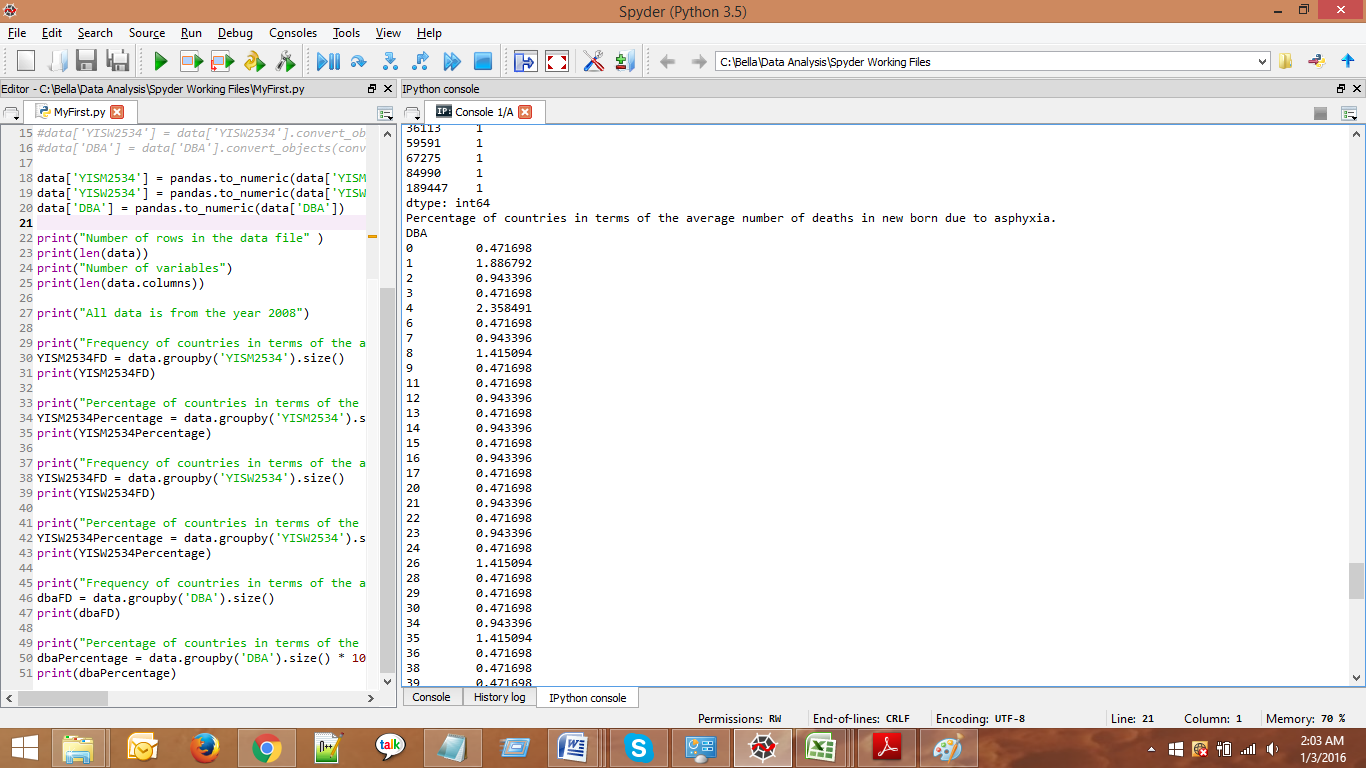
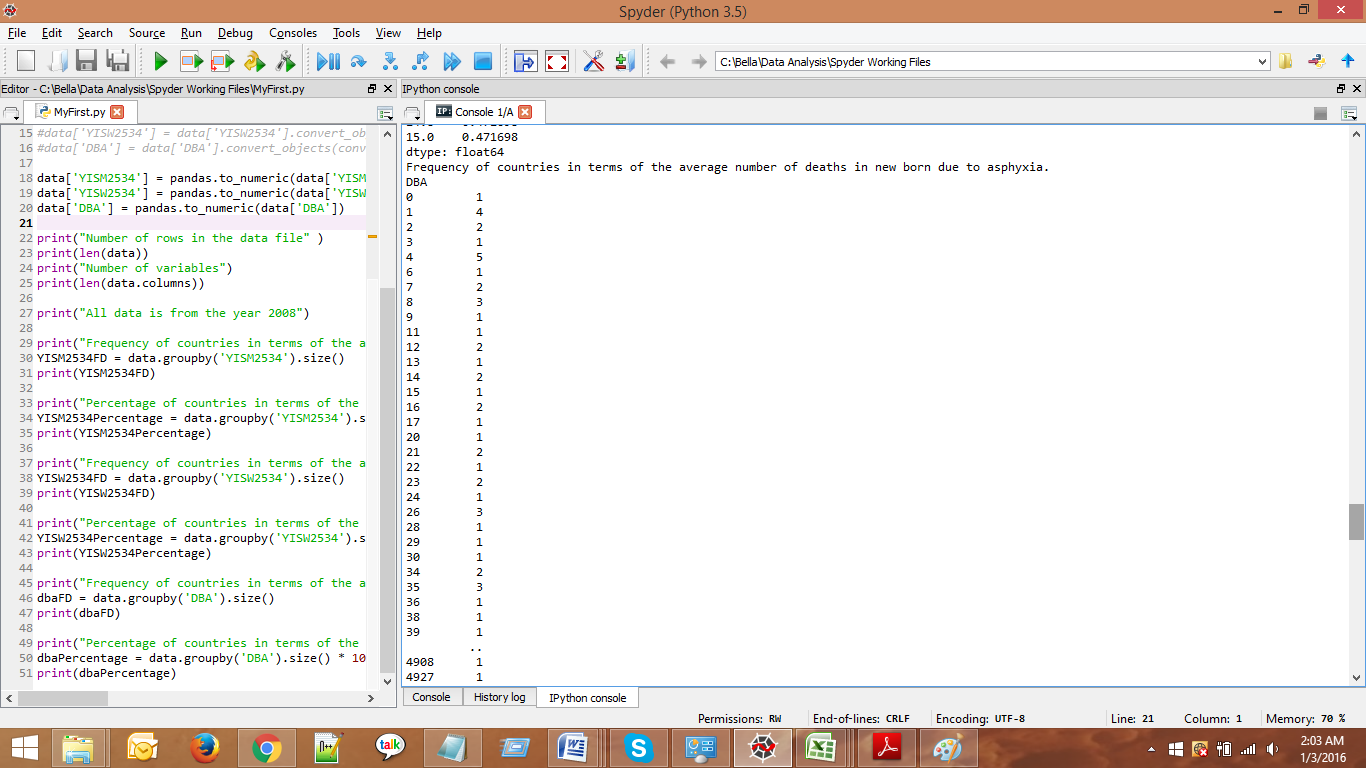
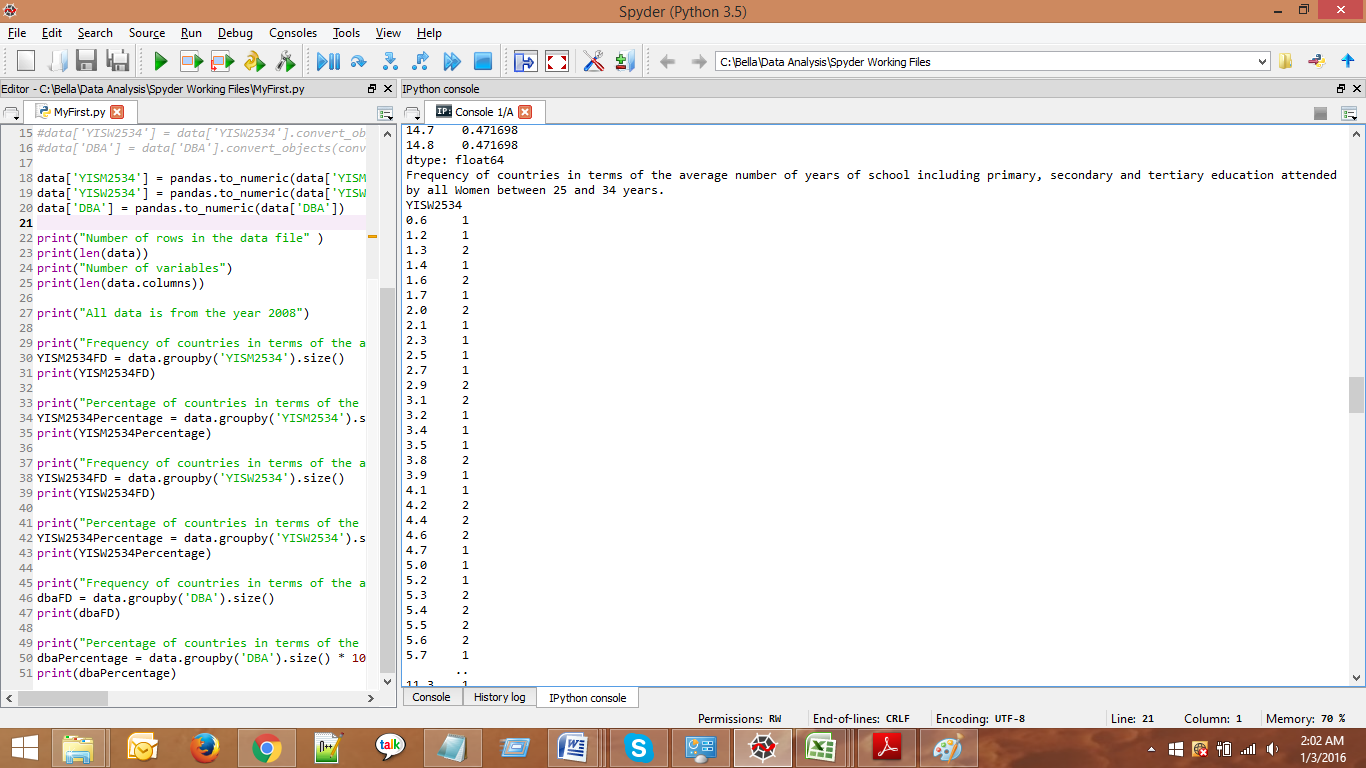
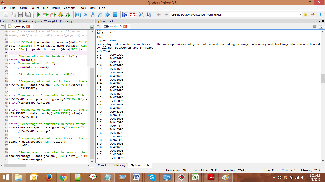
Screen shots of the results

Screenshot2 Screenshot7 Screenshot6 Screenshot5 Screenshot4 Screenshot3


In the above program, I have analyzed the frequency distribution of three variables:

YISM2534 :

The average number of years of school attended by all people in the age and gender group specified, including primary, secondary and tertiary education.

Since the variable takes an infinite number of values, it is not possible to summarize the results. Taking only the first three lines of the results (frequency and percentage) as a sample, it can be interpreted as follows:

YISM2534 (frequency)

2.6     2 (In two of the countries, the average years of education for men between the age group 25 and 34 is 2.6 years)

2.9     1 (In one country, the average years of education for men between the age group 25 and 34 is 2.9 years)

3.3     2 (In two of the countries, the average years of education for men between the age group 25 and 34 is 3.3 years)

—–

YISM2534 (Percentage)

2.6     0.943396 (In 0.94% of the countries, the average years of education for men is 2.6 years)

2.9     0.471698 (In 0.74% of the countries, the average years of education for men is 2.9 years)

3.3     0.943396 (In 0.94% of the countries, the average years of education for men is 3.3 years)

YISMW2534

The average number of years of school attended by all people in the age and gender group specified, including primary, secondary and tertiary education.

Since the variable takes an infinite number of values, it is not possible to summarize the results. Taking only the first three lines of the results (frequency and percentage) as a sample, it can be interpreted as follows:

YISM2534 (frequency)

0.6     1   (In one country, the average years of education for women between the age group 25 and 34 is 0.6 years)

1.2     1 (In one country, the average years of education for women between the age group 25 and 34 is 1.2 years)

1.3     2  (In two of the countries, the average years of education for women between the age group 25 and 34 is 1.3 years)

YISM2534 (Percentage)

0.6     0.471698 (In 0.47% of the countries, the average years of education for women is 0.6 years)

1.2     0.471698 (In 0.47% of the countries, the average years of education for women is 1.2 years)

1.3     0.943396 (In 0.94% of the countries, the average years of education for women is 1.3 years)

DBA:

Number of new borns that died specifically of asphyxia

Since this variable also takes an infinite number of values, it is not possible to summarize the results. Taking only the first three lines of the results (frequency and percentage) as a sample, it can be interpreted as follows:

DBA (frequency)

0     1  (In one country, the number of deaths by asphyxia is 0)

1     4 (In four of the countries, the number of deaths by asphyxia is 1)

2     2  (In two of the countries,the number of deaths by asphyxia is 2)

DBA (Percentage)

0         0.471698 (in 0.47% of the countries, there were 0 deaths by asphyxia)

1         1.886792 (in 1.8% of the countries, there was 1 deaths by asphyxia)

2         0.943396 (in 0.94% of the countries, there were 2 deaths by asphyxia)

As already mentioned, since none of the variables were categorical in nature, it was not possible to draw meaningful information from the data using only the frequency analysis.

Posted in Big Data, Data Analysis | Leave a comment

My First Project

Understanding the socio-economic factors of a specific region and how these factors influence each other is crucial to framing societal problems in the right context and finding constructive solutions. Aside from the obvious advantages and positive impact that such research can have, it also has the potential to open up new and innovative business opportunities. It is also a well-known fact that socio-economic factors hugely influence purchase behaviours amidst specific populations.

Since my primary reason for enrolling in this course is to ultimately learn how to interpret data in a way that is meaningful for businesses and consequently make informed decisions, I am interested in choosing a data set from GapMinder.

The GapMinder has a huge collection of socio-economic indicators from across the world.

Data Set Selected : GapMinder [http://www.gapminder.org/data/]

Primary Research Question: Is asphyxia death in newborns associated with births attended by skilled health staff?

Past research and inference

Skilled health staff at birth is associated with decreased neonatal mortality[1] as well as maternal mortality[2] in many regions. I would like to examine if death in newborns caused specifically by asphyxia is similarly negatively correlated to births attended by skilled health staff.

Following my primary research question, I would also like to examine the factors influencing the use of skilled birth attendants.

The presence of a skilled health staff at birth is a crucial element in neonatal health. A study of determinants of use of skilled birth attendant at delivery in Makueni,  Kenya[3] concluded that there is a positive correlation between a woman’s education level, partner’s education level, and the utilization of skilled delivery.

Therefore I expect a similarly positive correlation between the utilization of skilled birth attendants and increased education attainment on a global scale. My follow-up research will therefore examine whether the utilization of skilled birth attendants is correlated to education attainment uniformly across the globe.

Follow-up Research Question : Is the number of births attended by skilled health staff associated with increased educational attainment in the population?

Variables Selected

I will be selecting the following variables from the data set for my research.

  • Births attended by skilled health staff (% of total)
  • Birth asphyxia deaths in newborn (per 1,000 births)
  • Birth asphyxia deaths in newborn (total deaths)
  • Mean years in school (men 25 to 34 years)
  • Mean years in school (men 25 years and older)
  • Mean years in school (women % men, 25 to 34 years)
  • Mean years in school (women 25 to 34 years)
  • Mean years in school (women 25 years and older)
  • Mean years in school (women of reproductive age 15 to 44)

Code Book

Variable name Description of Indicator Main Source
Births attended by skilled health staff (% of total) Births attended by skilled health staff are the percentage of deliveries attended by personnel trained to give the necessary supervision, care, and advice to women during pregnancy, labor, and the postpartum period; to conduct deliveries on their own; and to care for newborns. Source: UNICEF, State of the World’s Children, Childinfo, and Demographic and Health Surveys by Macro International. World Bank
neonatal-Birth asphyxia GapMinder
Mean years in school (men between 25 and 34 years old) The average number of years of school attended by all people in the age and gender group specified, including primary, secondary and tertiary education. Institute for Health Metrics and Evaluation
Mean years in school (men 25 and older) The average number of years of school attended by all people in the age and gender group specified, including primary, secondary and tertiary education. Institute for Health Metrics and Evaluation
Mean years in school (women aged 25 to 34 as % men of same age) The average number of years of school attended by all people in the age and gender group specified, including primary, secondary and tertiary education. Institute for Health Metrics and Evaluation
Mean years in school (women between 25 and 34 years old) The average number of years of school attended by all people in the age and gender group specified, including primary, secondary and tertiary education. Institute for Health Metrics and Evaluation
Mean years in school (women 25 and older) The average number of years of school attended by all people in the age and gender group specified, including primary, secondary and tertiary education. Institute for Health Metrics and Evaluation
Mean years in school (women of reproductive age, 15 to 44) The average number of years of school attended by all people in the age and gender group specified, including primary, secondary and tertiary education. Institute for Health Metrics and Evaluation


References

Singh, K., Brodish, P., & Suchindran, C. (2014). A Regional Multilevel Analysis: Can Skilled Birth Attendants Uniformly Decrease Neonatal Mortality?Maternal and Child Health Journal18(1), 10.1007/s10995–013–1260–7. http://doi.org/10.1007/s10995-013-1260-7

BMC Pregnancy and Childbirth (2014) 10.1186/1471-2393-14-311

Gitimu, A., Herr, C., Oruko, H., Karijo, E., Gichuki, R., Ofware, P., … Nyagero, J. (2015). Determinants of use of skilled birth attendant at delivery in Makueni, Kenya: a cross sectional study. BMC Pregnancy and Childbirth15, 9. http://doi.org/10.1186/s12884-015-0442-2

Reference Links

Posted in Big Data, Data Analysis | Leave a comment

Data Management and Visualization

Data Management, Analysis, and Visualization

Data management, analysis, and visualization are crucial components in making informed business decisions. In the following weeks, I will be undertaking a new project in data management and visualization and documenting my progress in this blog. Stay tuned!

Posted in Big Data | Tagged , , | Leave a comment

No audio output device is installed – Windows XP


The problem:

1. You are seeing a red x near your speaker icon.


2. When you move your cursor atop the speaker icon, you get the message “No Audio Output Device installed”.

The solution:

First, don’t panic. There is a good chance that your audio output device has only been disabled and not been uninstalled. If it is disabled, simply enable it and it will work. Here’s how to do it.

Right click on your speaker icon and choose ‘Playback Devices’. Your speaker should show as disabled. Right click on Speakers and choose Enable. Your audio should be restored successfully.


Sometimes, if your speaker is disabled, it may not show on the window like this.

In this case, right click inside the window, and choose ‘Show Disabled Devices’. You should then be able to see the speakers. Right click again and choose ‘Enable’.

Now, if your speakers weren’t just disabled, you may have to try upgrading the drivers. If that’s the case, do the following.

Go to Start – > Control Panel -> Device Manager.

Look for Sound, Video, and game controllers. Click the + on the left.

You should see your audio device listed. For me it was High Definition Audio Device. It could be others like Realtek Audio Device for you. Anyway, right click on the audio device and select “Update Driver Software”.

    If your audio device was previously working, but not working now, you should be able to update the driver software from a local directory or from the Windows Vista CD. So choose ‘Browse my computer for driver software’.

      Select “Let me pick from a list of device drivers on my computer.

        Select your audio device driver from the list and click ‘Next’.

          Choose ‘Yes’ when the update driver warning pops up. Once the driver is updated, your audio device should start working again!


            Posted in How Tos | Tagged , , , , , , , , , | Leave a comment

            Partitioning in Windows Vista

            Partitioning in Windows Vista

            Partitioning a disk in windows vista is tricky business. I recently went through the exercise so I could install Ubuntu on my laptop and it took all of two days for what should have taken a few minutes. So I am documenting my efforts here and hopefully it will help somebody else  save time.

            Platform Information

            My efforts were on a Sony Vaio laptop with Windows Vista Home Premium installed on it. The hard disk was 10 GB with 40 GB of free space on a single partition.

            Partition using disk management

            It is recommended that the disk has at least 10 GB of free space for installing Ubuntu. Since I had more than enough, I decided to create a new partition with 25GB space.

            Creating a new partition in Vista is simple:

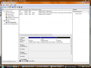
            1. Right click on my computer and click ‘manage’
            2. Click ‘continue’ when the user account control window pops up
            3. When the control panel->system window opens up, click the ‘disk management’ tab under storage.
            4. Click on the drive that you want to partition. Right click and choose the ‘shrink volume’ tab.
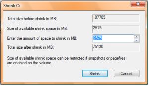
            5. It will take a few seconds for Vista to figure out how much space is available for creating the new partition. At this point, if you are lucky, Vista will show you the full space that is available as free space for shrinking. Go ahead and enter the space you need for Ubuntu and click ‘ok’. A new partition will be created with the space you entered and will be listed ‘Unallocated’.Partitioning Vista
            6. Right click on the partition and choose ‘New Simple Volume’
            7. Partitioning in VistaThe New Simple Volume Wizard will open up. Click ‘Next’ on the first screen. The second screen will ask you to choose a drive letter. Choose a letter that is not already assigned to any of your drives. Click ‘Next’.Partitioning in Vista
            8. If you are partitioning because you want to install Ubuntu, choose ‘Do not format this volume’. When you are done, it will show as a RAW partition. Otherwise, format it as NTFS.

            Formating a Vista Partition

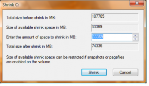
            Unfortunately, I was not so lucky. When I did the ‘shrink volume’, this is what I saw. I ran a windows defragmentation. The results were only marginally better. This time, I saw that I had 2 GB available. It was still not enough to make a Linux partition.

            Vista partitioning

            After much research (Thanks to Richard Baxter from www.SEOgadget.co.uk for pointing me in the right direction), I have compiled here the various solutions I tried before resolving the problem. I have tried to provide explanations for each step so that even if you run into problems that I did not encounter, you will still be able to find a way out. Hopefully, at the end of following these instructions, you will be able to reclaim all the free space available for shrinking the volume.

            Why can’t we shrink the volume?

            Windows Vista will be unable to claim free space for a new partition if there are system files scattered around in the free space. Before we see what files are blocking the disk, it would be easier if we simply delete some of the system files that in general take up a lot of space and don’t defragment easily.

            Delete system files and free up more space:

            Before creating a new partition, free up as much space from your hard disk as possible.

            Uninstall Unnecessary Applications

            Take this opportunity to uninstall all the applications that you don’t use anymore. This will free up quite a bit of free space.

            Disable Hibernation

            The hibernation file is a system file that stores hibernation information including any data contained in the memory, CPU and registers. This file is often huge and may take up close to 10GB of hard disk space. To make sure this file is not blocking the disk, disable hybernation.

            1. Open a command prompt window as administrator
              1. i.      Click start -> type in ‘cmd’ in the search box ->press ctrl+shift+enter
              2. ii.      Click the ‘continue’ tab in the user account control window
            2. In the command prompt, type

            powercfg –h off

            Disable Paging

            The pagefile is a portion of the hard disk that is used in addition to the RAM to temporarily store and retrieve files and thus speed up your computer. The space allocated for pagefile can be resized. Alternately, you can also disable pagefile so that the entire space on the hard disk allocated for pagefile is freed up. To disable pagefile:

            1. Right click on ‘My Computer’ and select ‘Properties’.
            2. Select ‘System Protection’.
            3. Click ‘Continue’ when the user account control window pops up.
            4. Click the ‘Advanced’ tab.
            5. Under ‘Performance’, click ‘Settings’.
            6. Go to the ‘Advanced’ tab and click ‘Change’.
            7. Uncheck ‘Automatically manage paging file size for all drives’.
            8. Select ‘No paging file’. Click ‘Set’ and then ‘Ok’

            Disable Paging in Vista

            After you disable the pagefile, it is advised that you do not run any other applications until your disk partitioning is completed successfully. This is because your system will then have to depend solely on the RAM for memory, which may not be enough, resulting in your applications getting crashed.

            Disable System Restore:

            System restore information is stored in system files called ‘system volume information’. They are stubborn and don’t get defragmented easily, Also, they often reside on the edge of the drive and prevent volume shrinking.

            There may be several system restore points in your computer. Let’s delete them all and disable system restore.

            1. Right click on ‘My Computer’ and select ‘Properties’.
            2. Select ‘System Protection’.
            3. Click ‘Continue’ when the user account control window pops up.
            4. Uncheck the drive for which you want to disable system restore.

            Disable System Restore in Vista

            Disable Kernel Memory Dump

            The kernel memory dump logs the contents of kernel memory when the computer stops unexpectedly. The size of the dump can vary anywhere from 150 MB to 2GB. To disable kernel memory dump,

            1. Right click on ‘My Computer’ and select ‘Properties’.
            2. Select ‘System Protection’.
            3. Click ‘Continue’ when the user account control window pops up.
            4. Click the ‘Advanced’ tab.
            5. Click ‘Settings’ under ‘startup and recovery’.
            6. Under ‘Write debugging information’, select (none). Click OK.

            Disable Kernel Memory Dump in Vista

            Run Disk Cleanup

            Now run the Windows disk cleanup tool.

            1. Select start->All Programs->Accessories->System Tools->Disk Cleanup.
            2. Select ‘Files from all users on this computer’
            3. Choose the ‘More Options’ tab.
            4. Under ‘System restore and shadow copies’, select ‘clean up’. Choose to delete all the previous restore points in the dialogue box that pops up.

            Defragment Using PerfectDisk

            PerfectDisk is a defragmenting software from Raxco and can be downloaded from their website: http://www.raxco.com/

            It is not free, but there is a 30 day free trial period. Download and install the latest version of PerfectDisk.

            Open PerfectDisk after installation. You will see that there are three options under which you can run defragmentation.
            1. Defrag only
            2. SMARTPlacement
            3. Consolidate Free Space

            Run defragmentation under all three options for the drive you wish to partition. When you are done, select the ‘Boot Time’ option. Reboot your computer and let PerfectDisk run. This way, PerfectDisk will be able to defragment some of the stubborn system files.

            When windows reboots, open PerfectDisk again and this time run ‘Analyze’. At this point, chances are that your drive has enough contiguous free space for partitioning and at the right location. If that is the case, go ahead and attempt to shrink volume again according to the instructions given in the beginning of this document.

            However, if it looked anything like the below, then, your ‘shrink volume’ will still show 0 GB for shrinking, even though your PerfectDisk shows a lot more as available largest free space chunk.

            Largest Freespace Chunk

            Vista Defragmenting

            In the above picture, the red boxeshighlight the fragmented blocks that are still blocking windows from being able to partition the drive. If this is what you are facing, there is more work to do before you can successfully partition the drive.

            Right click on the colored blocks to find out what files are located in the blocked area.

            • Rarely modified/Occasionally modified/recently modified/Directory/Boot: If the files that are blocking contiguous free space are from any of the above category, run defragmentation over and over again until the files move up to the top of the map.
            • If you see metadata scattered around in the free space, run the defragmentation again in ‘Boot Time’ mode. This will defragment most of the meta data. If after defragmenting, you still encounter meta data, right click on the block to see the file name names. Then delete the files manually. You may have to do this in the administrator mode.
            • If ‘Excluded’ files are blocking free space, then right click to see the file names. If it says ‘System Volume Information’, make sure that all the system restore points are deleted and system restore is disabled completely. Then run the defragmentation again.
            • If MFT files are fragmented and blocking free space, run defragmentation again in SMARTPlacement mode. If that does not work, try a different defragmenting program. Mydefrag (http://www.mydefrag.com/) is a freeware application that is worth a try. However, after you run Mydefrag, your MFT files may get defragmented, but your other files may be in a disarray. So run PerfectDisk again, as many times as needed until you are satisfied.

            I was able to finally make my disk look like this at the end of the above exercise.

            Vista Partitioning

            Hopefully, you will too!

            Posted in How Tos | Leave a comment

            Remembering Jules Verne

            No. It is not his birthday. In fact, it is a whole two months after his birthday. But I was doing my spring cleaning and happened to come across a copy of Verne’s “A journey to the centre of the earth”. My thoughts began to wander. It has been years since I read a book by Jules Verne. But the fascination remains as fresh as the day light at dawn.

            Jules Verne was a French man born in the early 19th century. To be more exact, he was born in 1828, in Nantes. When in 1851, he published his first novel, “Cinq semaines en ballon (five weeks in a balloon)”, it was still the early days of balloon making. But the book was in no way a mere fantasy of the author. Instead, it involved a serious research into geology, engineering and astronomy.

            The world’s first balloon, carrying people, was launched in 1783, as an experiment by Messrs. Charles and Robert. Benjamin Franklin, the American Scientist who is today, well known for his kite experiment, recorded the event in his letter to Sir Joseph Banks. In his letter, he states that the balloon rose to about 800 feet from the ground, and carried with it Mr. Charles, an experimental philosopher, and monsieur Robert, one of the constructors of the balloon. These were the early days of synthetic balloons, until which time balloons were the product of animal bladders. This incident was probably what triggered Verne to write his first novel, in which one Dr. Ferguson initiates a voyage to Africa in a balloon.

            “Five weeks in a balloon” was the beginning of Verne’s journey into the future. Although the idea of traveling in balloons themselves had already been done, the book, predicts some of the greatest events to come. In the first chapter of the book, Elspeth, Dr. Ferugson’s confidential maid remarks at the idea of his balloon voyage thus.

            “Not a bit of it!” said she. “Don’t I know my man? Isn’t it just like him? Travel through the air! There, now, he’s jealous of the eagles, next! No! I warrant you, he’ll not do it! I’ll find a way to stop him! He! why if they’d let him alone, he’d start some day for the moon!”

            Fourteen years hence, Verne wrote the book, “From the Earth to the Moon”. In the book, a Baltimore gun company embarks on a mission to make the ultimate gun that can launch a manned rocket to the moon. This was in 1865, when even aeroplanes did not exist.

            After 99 years the Apollo 11 landed on the moon with Edwin Aldwin and Neil Armstrong of America. With thoughts that were a whole century ahead of his world, what is fascinating about the book is the intense amount of detail that Verne gives the reader, when none of the details existed. Beginning from the material chosen to build the projectile, all the way to its dimensions, the force required for the projection, and the amount of gun powder necessary for impulsion, the novel gives a detailed description.

            Come to think of it, ‘A journey to the centre of the earth’ is probably one of his few fantasies that is yet to be realized. Is it even necessary to visit the centre of the earth? But as history teaches us, it is only a matter of time before the fantastic becomes reality for whatever reason.

            Posted in Science Fiction, Uncategorized | Tagged , , , | Leave a comment

            QR Codes

            What are QR Codes

            QR code stands for Quick Response Code. QR codes are 2-dimensional bar codes that can be used to embed data. The data can be any of the following:

            1. Numbers
            2. Alphabets
            3. Special Characters
            4. Kanji Characters
            5. FNC1 data

            You can read the data contained within a QR code either with a QR code reader or with a mobile phone equipped with a QR code reader. There are two types of QR codes.

            1. Micro QR codes: A micro QR code can hold only limited data. It has a single finder pattern (the black-white-black box) on the top left corner of the symbol. There are 4 versions of micro QR codes – M1, M2, M3 and M4.

            2. QR code 2005 symbol: It can hold more data than the micro QR code and has the full range of capabilities. It has 3 finder patterns, one on the top left corner, one on the top right corner and the third on the bottom left corner. There are 40 versions of QR code 2005 symbols.

            What can you do with QR Codes

            1. One of the coolest things you can do with QR codes is embed URLs. Upon decoding the QR code, the user will be directed to the URL contained within the symbol. This way, you can provide quick information to the user regardless of where he is.

            Other uses for QR codes include:

            2. Encouraging quick action from a user in response to advertisements, promotions, events and shows. For example,  a decoded QR code can direct users to a website for buying tickets to an event.

            3. Executing specific instructions upon reading the code. For example, A QR code when decoded, can  send an automatic e-mail to a specific address.

            Posted in QR Codes | Leave a comment