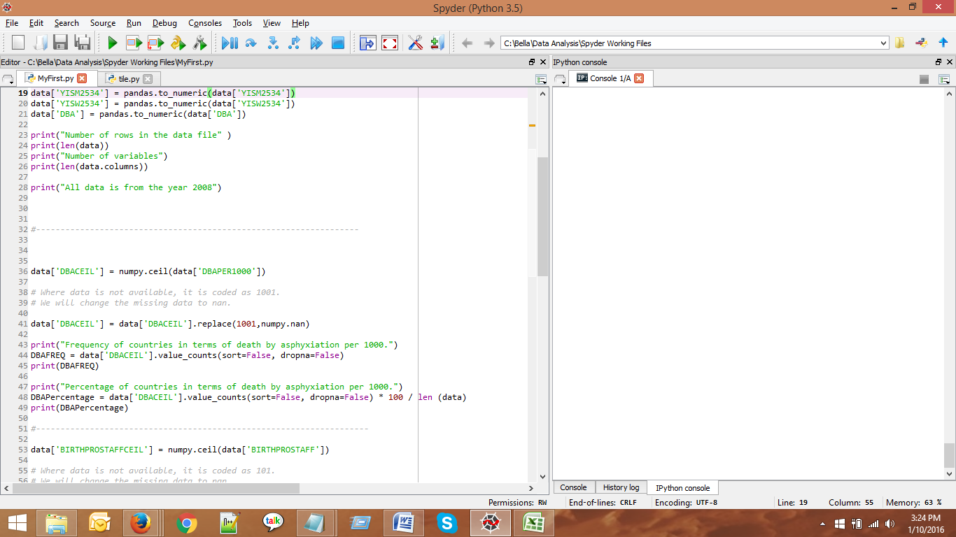
In my previous post, I had performed a frequency analysis on three of the variables from my data set:
YISM2534: Mean years in school (men between 25 and 34 years old)
YISW2534: Mean years in school (women between 25 and 34 years old)
DBA: Asphyxia deaths in newborn (total deaths)
The analysis was not friendly to interpretation due to the variables taking infinite number of values. Therefore, I have made some changes to the data to make it more interpretable.
- First, I have also included a fourth variable for my analysis: BIRTHPROSTAFF: Total number of births attended by professional staff. I have included BIRTHPROSTAFF as it pertains directly to my primary research question.
- Second, I have changed the variable DBA to DBAPer1000 (death by asphyxia per 1000) since this variable accounts for the variations in population size among the different countries whereas DBA does not do so.
- Third, I have set aside missing data in each of the variables
- YISM2534: Missing data was coded as 0. It has been changed to nan.
- YISF2534: Missing data was coded as 0. It has been changed to nan.
- DBAPER1000: Missing data was coded as 1001. It has been changed to nan.
- BIRTHPROSTAFF: Missing data was coded as 101. It has been changed to nan.
- Since each of the variables took infinite number of values (float), frequency analysis did not yield any meaningful data in the earlier run. Therefore, to make the frequency analysis more meaningful, I created secondary variables for each of my chosen variables. The secondary variables are basically the ceiling values of the primary variables. After the conversion, YISM2534 and YISW2534 now take integer values from 1 to 15 without decimals. Similarly, I applied the ceiling function to DBAPER1000 and BIRTHPROSTAFF. This exercise has yielded a more interpretable frequency and percentage analysis for all variables.
- I have created a new data frame dataNew using the secondary variables. In my output, I have printed the first 25 rows of this new data frame.
- There are no skip patterns in my data set and therefore there is no need to manage skip patterns
- All variables take quantitative values and therefore coded logically. Therefore, none of them required recoding.
Code:
# -*- coding: utf-8 -*-
“””
Spyder Editor
This is a temporary script file.
“””
# This is my “Hello World Code”
import pandas
import numpy
import math
data = pandas.read_csv(‘data.csv’)
#data[‘YISM2534’] = data[‘YISM2534’].convert_objects(convert_numeric=True)
#data[‘YISW2534’] = data[‘YISW2534’].convert_objects(convert_numeric=True)
#data[‘DBA’] = data[‘DBA’].convert_objects(convert_numeric=True)
data[‘YISM2534’] = pandas.to_numeric(data[‘YISM2534’])
data[‘YISW2534’] = pandas.to_numeric(data[‘YISW2534’])
data[‘DBA’] = pandas.to_numeric(data[‘DBA’])
print(“Number of rows in the data file” )
print(len(data))
print(“Number of variables”)
print(len(data.columns))
print(“All data is from the year 2008”)
#——————————————————————
data[‘DBACEIL’] = numpy.ceil(data[‘DBAPER1000’])
# Where data is not available, it is coded as 1001.
# We will change the missing data to nan.
data[‘DBACEIL’] = data[‘DBACEIL’].replace(1001,numpy.nan)
print(“Frequency of countries in terms of death by asphyxiation per 1000.”)
DBAFREQ = data[‘DBACEIL’].value_counts(sort=False, dropna=False)
print(DBAFREQ)
print(“Percentage of countries in terms of death by asphyxiation per 1000.”)
DBAPercentage = data[‘DBACEIL’].value_counts(sort=False, dropna=False) * 100 / len (data)
print(DBAPercentage)
#——————————————————————–
data[‘BIRTHPROSTAFFCEIL’] = numpy.ceil(data[‘BIRTHPROSTAFF’])
# Where data is not available, it is coded as 101.
# We will change the missing data to nan.
data[‘BIRTHPROSTAFFCEIL’] = data[‘BIRTHPROSTAFFCEIL’].replace(101,numpy.nan)
print(“Frequency of countries in terms of births attended by professional staff.”)
BIRTHPROSTAFFFREQ = data[‘BIRTHPROSTAFFCEIL’].value_counts(sort=False, dropna=False)
print(BIRTHPROSTAFFFREQ)
print(“Percentage of countries in terms of births attended by professional staff.”)
BIRTHPROSTAFFPercentage = data[‘BIRTHPROSTAFFCEIL’].value_counts(sort=False, dropna=False) * 100 / len (data)
print(BIRTHPROSTAFFPercentage)
#—————————————————————–
data[‘YISM2534CEIL’] = numpy.ceil(data[‘YISM2534’])
# Where data is not available, it is coded as 0.
# We will change the missing data to nan.
data[‘YISM2534CEIL’] = data[‘YISM2534CEIL’].replace(0,numpy.nan)
print(“Frequency of countries in terms of the average number of years of school including primary, secondary and tertiary education attended by all men between 25 and 34 years.”)
YISM2534FREQ = data[‘YISM2534CEIL’].value_counts(sort=False, dropna=False)
print(YISM2534FREQ)
print(“Percentage of countries in terms of the average number of years of school including primary, secondary and tertiary education attended by all men between 25 and 34 years.”)
YISM2534Percentage = data[‘YISM2534CEIL’].value_counts(sort=False, dropna=False) * 100 / len (data)
print(YISM2534Percentage)
#—————————————————————-
data[‘YISW2534CEIL’] = numpy.ceil(data[‘YISW2534’])
#print(YISM2534FLOOR)
# Where data is not available, it is coded as 0.
# We will change the missing data to nan.
data[‘YISW2534CEIL’] = data[‘YISW2534CEIL’].replace(0,numpy.nan)
print(“Frequency of countries in terms of the average number of years of school including primary, secondary and tertiary education attended by all women between 25 and 34 years.”)
YISW2534FREQ = data[‘YISW2534CEIL’].value_counts(sort=False, dropna=False)
print(YISW2534FREQ)
print(“Percentage of countries in terms of the average number of years of school including primary, secondary and tertiary education attended by all women between 25 and 34 years.”)
YISW2534Percentage = data[‘YISW2534CEIL’].value_counts(sort=False, dropna=False) * 100 / len (data)
print(YISW2534Percentage)
#———————————————————————
# Print the new dataframe that contains the ceiling values
dataNew = data[[‘Countries’,’YISM2534CEIL’, ‘YISW2534CEIL’, ‘DBACEIL’, ‘BIRTHPROSTAFFCEIL’ ]]
print(dataNew.head(25))
#———————————————————————-
Output:
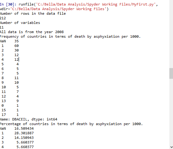
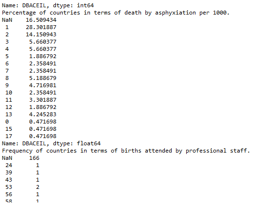
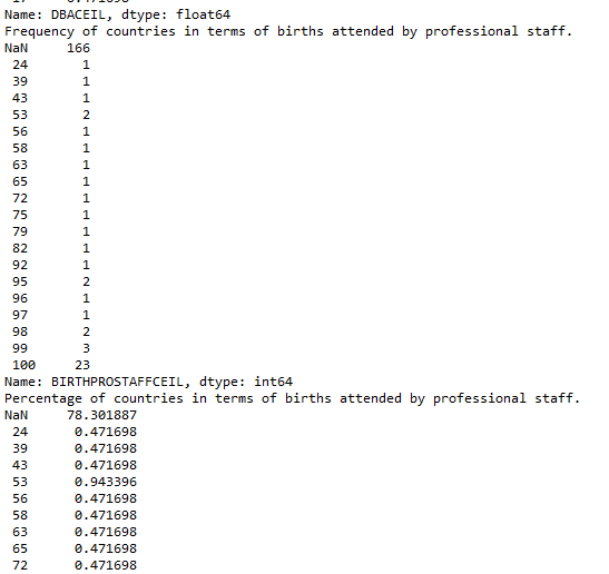
Now that the data has been managed, the frequency analysis on each of the variables is more interpretable. For example, when considering death by asphyxia per 1000 data, the majority of the countries have a low number – 60 countries have only one recorded death per 1000, 30 countries have only 2 recorded deaths per 1000 and so on. The frequency analysis similarly show meaningful data for the other selected variables.
Output in case the screenshot is not clear:
runfile(‘C:/Bella/Data Analysis/Spyder Working Files/MyFirst.py’, wdir=’C:/Bella/Data Analysis/Spyder Working Files’)
Number of rows in the data file
212
Number of variables
11
All data is from the year 2008
Frequency of countries in terms of death by asphyxiation per 1000.
NaN 35
1 60
2 30
3 12
4 12
5 4
6 5
7 5
8 11
9 10
10 5
11 7
12 4
13 9
0 1
15 1
17 1
Name: DBACEIL, dtype: int64
Percentage of countries in terms of death by asphyxiation per 1000.
NaN 16.509434
1 28.301887
2 14.150943
3 5.660377
4 5.660377
5 1.886792
6 2.358491
7 2.358491
8 5.188679
9 4.716981
10 2.358491
11 3.301887
12 1.886792
13 4.245283
0 0.471698
15 0.471698
17 0.471698
Name: DBACEIL, dtype: float64
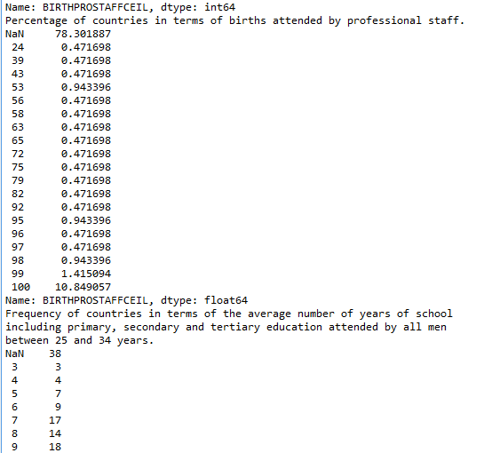
Frequency of countries in terms of births attended by professional staff.
NaN 166
24 1
39 1
43 1
53 2
56 1
58 1
63 1
65 1
72 1
75 1
79 1
82 1
92 1
95 2
96 1
97 1
98 2
99 3
100 23
Name: BIRTHPROSTAFFCEIL, dtype: int64
Percentage of countries in terms of births attended by professional staff.
NaN 78.301887
24 0.471698
39 0.471698
43 0.471698
53 0.943396
56 0.471698
58 0.471698
63 0.471698
65 0.471698
72 0.471698
75 0.471698
79 0.471698
82 0.471698
92 0.471698
95 0.943396
96 0.471698
97 0.471698
98 0.943396
99 1.415094
100 10.849057
Name: BIRTHPROSTAFFCEIL, dtype: float64
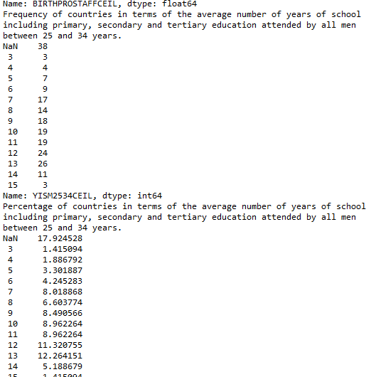
Frequency of countries in terms of the average number of years of school including primary, secondary and tertiary education attended by all men between 25 and 34 years.
NaN 38
3 3
4 4
5 7
6 9
7 17
8 14
9 18
10 19
11 19
12 24
13 26
14 11
15 3
Name: YISM2534CEIL, dtype: int64
Percentage of countries in terms of the average number of years of school including primary, secondary and tertiary education attended by all men between 25 and 34 years.
NaN 17.924528
3 1.415094
4 1.886792
5 3.301887
6 4.245283
7 8.018868
8 6.603774
9 8.490566
10 8.962264
11 8.962264
12 11.320755
13 12.264151
14 5.188679
15 1.415094
Name: YISM2534CEIL, dtype: float64
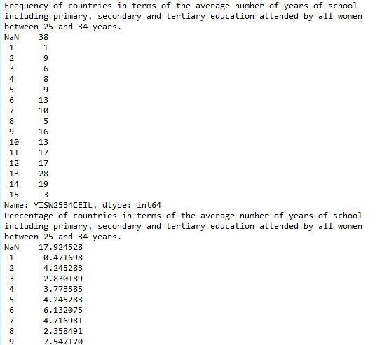
Frequency of countries in terms of the average number of years of school including primary, secondary and tertiary education attended by all women between 25 and 34 years.
NaN 38
1 1
2 9
3 6
4 8
5 9
6 13
7 10
8 5
9 16
10 13
11 17
12 17
13 28
14 19
15 3
Name: YISW2534CEIL, dtype: int64
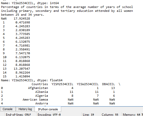
Percentage of countries in terms of the average number of years of school including primary, secondary and tertiary education attended by all women between 25 and 34 years.
NaN 17.924528
1 0.471698
2 4.245283
3 2.830189
4 3.773585
5 4.245283
6 6.132075
7 4.716981
8 2.358491
9 7.547170
10 6.132075
11 8.018868
12 8.018868
13 13.207547
14 8.962264
15 1.415094
Name: YISW2534CEIL, dtype: float64
Countries YISM2534CEIL YISW2534CEIL DBACEIL \
0 Afghanistan 4 1 13
1 Albania 11 11 1
2 Algeria 8 7 6
3 American Samoa NaN NaN NaN
4 Andorra NaN NaN NaN
5 Angola 7 5 13
6 Antigua and Barbuda 14 14 NaN
7 Argentina 12 12 1
8 Armenia 12 12 3
9 Aruba NaN NaN NaN
10 Australia 13 13 1
11 Austria 13 12 1
12 Azerbaijan 13 13 4
13 Bahamas 12 13 2
14 Bahrain 11 12 1
15 Bangladesh 6 5 10
16 Barbados NaN NaN 2
17 Belarus 13 13 1
18 Belgium 13 14 1
19 Belize 10 10 2
20 Benin 5 3 8
21 Bermuda NaN NaN NaN
22 Bhutan NaN NaN 9
23 Bolivia 11 10 7
24 Bosnia and Herzegovina 11 10 2
BIRTHPROSTAFFCEIL
0 24
1 NaN
2 NaN
3 NaN
4 NaN
5 NaN
6 100
7 95
8 100
9 NaN
10 NaN
11 NaN
12 NaN
13 NaN
14 98
15 NaN
16 NaN
17 100
18 NaN
19 95
20 NaN
21 NaN
22 NaN
23 72
24 NaN

